In many scientific applications there is a need to build a 2D map of some value, kind of 2D distribution or strictly speaking 2D function. Most of the time the area is discrete, i.e. pixelated. Often it is done in one 2D picture using density plot, where the value of function at point x,y is represented by the brightness of the pixel with coordinates x and y. In superresolution localization microscopy resulting pictures are often rendered as 2D “probability density functions”. I.e. each pixel’s brightness reports a probability to observe some number of molecules at given volume, taken from some measurements (microscopy acquisition). But what should be done if one wants to show on the same picture two 2D functions simultaneously? For example, for localization microscopy, combine probability and also Z-coordinate?
It is quite general question, how to simultaneously visualize two 2D functions. For example, height of some terrain and average density of trees on a map. Or some energy distribution and density of particles over a space. One widespread approach used is to code one variable with brightness and another with color. In this post I would try to explore this question (mostly for myself) on example of STORM/PALM colorcoded rendering.
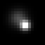
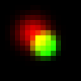
I start with a simple example, rendering of two overlapping particles. The probability plot is usually built in localization microscopy field as illustration. For each particle localized the area under surface is always normalized and so width/height of particle depends on localization precision. Usually only black and white gradations are used (called grayscale). In the following GIF I show two particles, one with good (bright, below) and another one with poorer localization (dim, above):
To plot them together it is quite logical to sum them up, i.e. sum up their brightness (picture contrast is adjusted on following image in comparison with previous two):
Notice that the bright spot is not symmetric anymore, since its top left corner is overlapped with the dim one and pixels intensities in the overlap added up. Now let’s try to add color to picture, since it is grayscale now and use color to code for the depth (z-coordinate of particle). Everywhere below I would use “spectrum” Lookup table, the one that codes depth with hue. Any other LUT can be used if proper indexing is performed. I assume that the dim spot is red, while the bright spot is green. One first simple way to render it is to just sum up all the R, G and B channels of the image. Here is how it will look like:
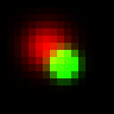
OPTION1
Looks ok, overlapping area is a bit yellow since red dim spot leaks a bit to the green bright. In this case the value of red channel intensity of overlapping pixel (where 


Also we can take maximum value in each of R, G and B channels independently and it would give almost the same result:

OPTION2
Formula describing intensity of red channel:

Another approach is to transform each color to HSB space. In short, instead of R, G and B levels we would have hue (kind of wavelength), saturation and brightness. It looks easy to work in this space, because now we can simply map probability to brightness and z-coordinate to hue (let’s leave saturation for now). So for overlapping pixels we always add up brightness (as we did for grayscale picture), now what to do with hue? One option is to assign the hue of brighter spot (maximum projection), here how it would look like:
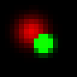
OPTION3
Obviously, green dot dominates overlap. Alternatively, instead of assigning the hue of spot with maximum brightness property (intensity), we can assign “weighted average” hue with weights being brighness of each spot at the current pixel. It will look like this:
OPTION4
It looks a bit strange in this simple example, but I think it is very promising approach. To illustrate this, let’s take a look at a bit more complicated case, when we have a real 3D SM data with big numbers of multiple overlapping spots (microtubules image data provided by Desiree, very talented postdoc in our lab). In absence of Z coordinate information they would look like this:
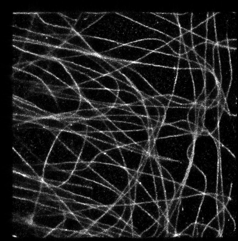
GRAYSCALE click to enlarge
Since I know final results, I would prefer to start with OPTION2.
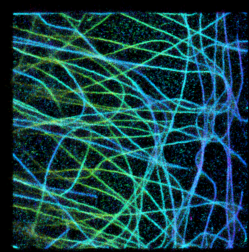
OPTION2 click to enlarge
The same result can be generated by rendering z-stack and applying “Temporal color-code” procedure in FIJI. Notice that there are a lot of “noisy” background around microtubules (curves) and since overlapping brightness of particles does not add up, summary brighness of microtubules is the same as individual spots of noise. It is almost exactly the same as:
OPTION3 click to enlarge
and exactly for the same reason. Dots intensities at background are on the same order as dots intensities on microtubule, since overlapping dots’ intensities on microtubules do not add up to each other (maximum intensity takes over).
Ok, so now let’s go to summing stuff up:
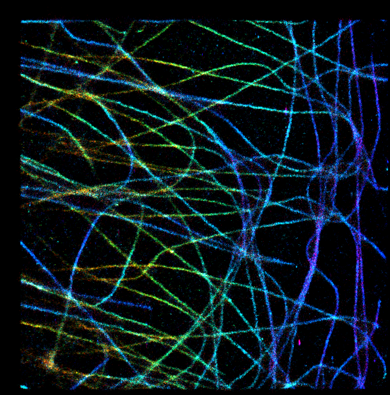
OPTION1 click to enlarge
Now it looks much better! Pooled intensities of overlapping spots on microtubules are brighter and they can “beat” the background. The only problem in my opinion is that the color of pixels with multiple overlapping spots now has changed. Suddenly red color appears at many green/yellow microtubules, making them appear at different height than the real data. It happens in dense areas, since each of R,G,B channel is summed up independently, so for example small amounts of red color can build up and manifest itself where it is not supposed to be. At least this is the most probable explanation that comes to my mind.
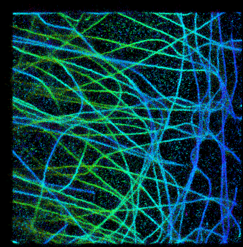
Now the last option:
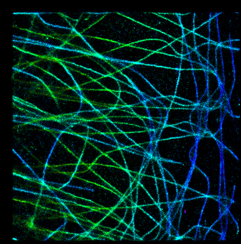
OPTION4 click to enlarge
In this case the color cannot be higher/lower than min and max hue of overlapping spots and red areas are missing. So I think this option is kind of optimal in terms of data representation.
0 Comments