//><=~!=//

First of all, here is link to part 1 and here is link to the video of my talk about applications of correlation.

This part is mostly technical, about correlation calculation approaches. In the end of the last post a “cross-correlation measure” was defined (not real cross-correlation) as the summary of Euclidean distances between two functions in 1D. For 2D (images) there are 2 independent space coordinates, so “cross-correlation distance” is also 2D function.

Essentially, for two images the distance (between intensities) needs to be calculated:

for all possible combinations of and . So explicit formula for the squared distance is:

where and intensity values of image1 and image2 at coordinates and . Now, following this paper (again), expanding the squared bracket gives:

First and last term seems to be constant, so we are interested only in the middle term. This is actually not true, since we calculating this sum only over overlapping area of both images. Non-overlapping areas are not defined. But we skip this for now (return to it in a minute) and focus on solving issue of normalization, described in the end of previous post. To overcome it, it is suggested to use normalized correlation coefficient, usually written as:

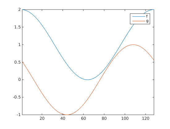
Ok, this is getting too complicated and bulky, let’s get back to a one-dimensional case:

Still huge, but a little more simple. What are the differences between this normalized correlation coefficient and “function distance” introduced earlier?

First of all, it changed its sign. It was negative for the term ( times ) inside “the distance”, now it is positive. Which means that if for the distance we were looking for the shift that provides the minimum value of the distance (corresponding to maximum similarity). Now, using the last definition, we should look for the maximum. It makes sense, looking for “maximum correlation”.

The second addition, the average value is subtracted from both functions before calculation of anything. This actually makes sense, to avoid situations demonstrated in the previous example (when one function has some offset). The idea is to compare signal/function shape, not an absolute value.

The third addition is the denominator. This expression was chosen specifically in this form, so that the cross-correlation coefficient’s value is always between one and minus one. For example, the value of normalized cross-correlation of the function with itself (autocorrelation) is equal to 1.

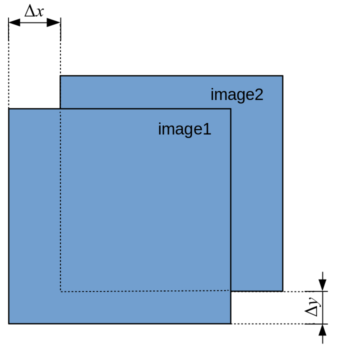
Now, in practical terms, usually, both functions are defined on some specific interval of . For example, here are two cosine functions shifted in x by value of 20 (f has additional y offset), defined on the interval from 1 till 128.

Now, when I shift one of them to calculate correlation, there are non-overlapping areas along , where multiplication is not defined:

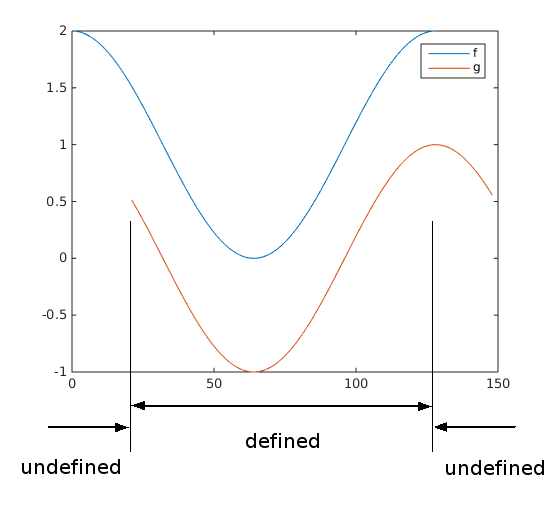
So how to make multiplication in the numerator outside of overlap? Usually, in this case, it is assumed that functions’ values outside the overlapping area are zeros, so these “tails” do not contribute to the numerator.
Corresponding normalized cross-correlation function will look like this (here is corresponding matlab code):

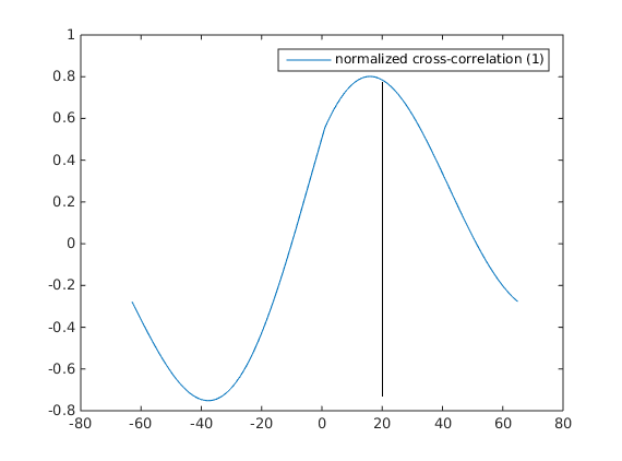
Looks fine, but there are some details. First, notice that the peak value of correlation is not equal to 1, although functions (after average subtraction) overlap perfectly! The reason for that is that for this shift the numerator multiplication is calculated over the corresponding overlap, while the denominator is calculated over the whole interval. So basically as the shift value of increasing, the multiplication is taken over smaller and smaller range in the numerator, while normalization coefficient in the denominator is taken over the whole constant interval. This leads to another problem.
The peak of cross-correlation is not exactly at the position. Since now it is a balance of shrinking interval vs correlation value.

So it is a good or a bad thing? I think, that it depends on the specific application of the cross-correlation function. If the most interesting thing is the degree of overall correlation between two functions, it is a good thing. It shows that only part of the shape is similar, encoding in the final value the length of “the interval of similarity”. But if one is looking for the very similar segments between two functions (like in the case of drift correction for microscopy, for example) it is not a good thing.

One obvious way to solve this problem is to calculate the normalization coefficient in the denominator only over the overlapping interval. This is how cross-correlation is going to look like in this case (and corresponding code):

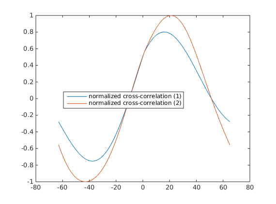
Now it is equal to 1 and peaks perfectly at .

Calculation of the numerator term is quite computationally demanding (and of the denominator according to the last definition too). To overcome this problem, different tricks are used (Fourier transform and integral table) with different limitations. The next post is going to be about them.