Whoa, almost nine years later, I finally decided to finish the story about cross-correlation. Just in case, here is part 1, part 2. This post is about the practical aspects of normalized cross-correlation (NCC) calculation. I will consider and compare different existing algorithms for this purpose and provide some technical details.
First, let’s see what is the required time complexity (number of required computations), if one wants to calculate the NCC in a direct, straightforward manner, according to the formula from the previous post.
For simplicity, I am going to assume that we are using two 1D/2D or 3D images with the same size of all dimensions (equal to n).
Direct (straightforward) calculation
Here is the formula for 1D, just as a reminder:
\(\displaystyle \gamma(\Delta x)=\frac{\sum_{x}[f(x)-\overline{f}_{x}][g(x-\Delta x)-\overline{g}_{x}]}{\sqrt{\sum_{x}[f(x)-\overline{f}_{x}]^2\sum_{x}[g(x-\Delta x)-\overline{g}_{x}]^2}}\)For the 1D case, assume we have two “images” or rows of numbers with n elements. Let’s estimate how many arithmetical operations we would need to calculate NCC for all possible shifts. We start with the shift of \(\Delta x = 0\), basically when these “row images” are not shifted with respect to each other.
see full derivation for 1D/2D/3D
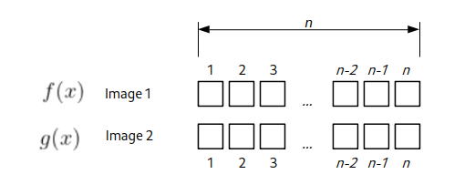
First, we would need to calculate the average values \(\overline{f}_{x}\) and \(\overline{g}_{x}\), which will take 2*n operations. Then we need to subtract this value from all elements (+ 2*n). For the denominator, we need to square each subtracted value (+ 2*n), make a sum (+ 2*n), multiply (+1), and take the square root (+1). For the numerator, we need to calculate the multiplication over the overlapping region of size n. And finally, perform division, but that is just one operation. All in all, one would need 9*n + 3 CPU operations for this shift value.
For the next shift value \(\Delta x = 1\), the overlapping region would be of (n-1) size.
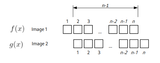
Using the same calculations as above, we would need 9*(n – 1) + 3 operations. Now it is clear where it is going. For the \(\Delta x = 2\) we would need 9*(n – 2) + 3 and so on. So basically, for a given shift, one would need \(9*(n-\Delta x)+3\) arithmetical operations. All possible shift values span from (-1)*(n – 1) till (n – 1). To get the total number of operations, we sum them up, and using the formula for the sum of the arithmetic progression, one can achieve:
\(\sum\limits_{\Delta x=-(n-1)}^{n-1}[9*(n-|\Delta x|)+3] = 9*n^2 + 3*(2n-1)=O(n^2)\)
So this is a precise formula, but in the computer science field, to get an idea about an algorithm’s complexity and performance depending on the input size n, people usually use “Big O notation” (wiki, explanation). In short, for each formula its just takes the “fastest growing term” and discards multiplications/additions of constants. In these terms, for the formula derived above the complexity is characterized as \(O(n^2)\), i.e. quadratic dependence of speed from the size of the input.
Now let’s do similar estimates for 2D, “regular” images. Suppose we have two images of equal size n x n. For the zero shift value \(\Delta x = 0\), \(\Delta y = 0\) we would need \(9*n^2 + 3\) calculations. Now for the shifts where one of the \(\Delta x\) , \(\Delta y \) is zero and another is plus/minus one, we would need \(9*n(n-1) + 3\) operations. Because in this case, the overlap area between the images would be smaller by one row or column. There are four of these shifts, see below.
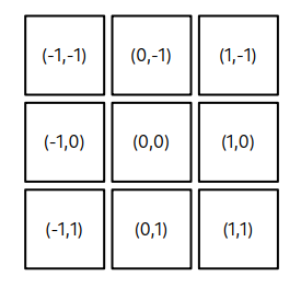
The shifts at the corners will require \(9*(n-1)^2 + 3\) operations. To make an estimate a bit simpler, let’s suppose that each square around (0,0) position would require approximately ~ \((n-1)^2\) and we need to calculate it 8 times. Let’s call this “squared circle” for the “general shift” value m = 1.
Extending the estimate for the next shift value “squared circle” of m = 2, it should be ~ \((n-2)^2\) operations. How many times do we need to calculate it? We can count these gray pixels on the picture below
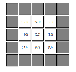
or we can derive a formula. For the shift m in one dimension, one size of the square is from –m till m, so it is \( 2m+1 \). The area would be \((2m+1)^2\). Now we need to subtract the area of the “inside” square corresponding to the shift of m-1, i.e. \((2(m-1)+1)^2\). This gives us
\((2m+1)^2 – (2m-1)^2 = 8m\)
Again, we want to perform the NCC calculation for the total range of m spanning from 1 to n-1, therefore in total we need to perform approximately (omitting constant factors):
\(\sum\limits_{m=1}^{n-1}[(n-m)^2*8m]=\frac{2}{3}(n-1)n^2(n+1) = O(n^4) \)
So for 2D images of size n we would need to perform \(O(n^4)\) operations.
For 3D volumetric images n x n x n we again expect ~ \((n-m)^3\) calculations per shift m and a total of \((2m+1)^3 – (2m-1)^3 = 24*m^2+2\) calculations (see above), giving the complexity of:
\(\sum\limits_{m=1}^{n-1}[(n-m)^3*m^2]=\frac{1}{60}n^2(n^4-1) = O(n^6) \)
So basically the complexity of the calculations is \(O(n^{2*D})\), where D is the number of dimensions. In other words, if we denote the total number of pixels in the image as \(N=n^D\), we would have \(O(N^2)\), which is just another way to look at the same things.
This observed quadratic complexity is pretty inefficient and generally considered computationally expensive. Specifically, if one needs to compute NCC for a 2D image twice the size (in both dimensions) of some reference, one would need to compute 16 times more operations, i.e., wait 16 times longer.
Therefore, the direct NCC correlation calculation algorithm is rarely used in practice, because it is so slow. Usually, alternative calculation methods are used; the most typical ones (to my knowledge) are outlined below.
Fast normalized cross-correlation
In 1995, J.P. Lewis presented an algorithm for fast calculation of the NCC. All the details are via the link (+ yeah, it was developed for the Forrest Gump movie!). I will briefly describe the main points of this seminal paper. Quick reminder, the formula for NCC of 1D images:
\(\displaystyle \gamma(\Delta x)=\frac{\sum_{x}[f(x)-\overline{f}_{x}][g(x-\Delta x)-\overline{g}_{x}]}{\sqrt{\sum_{x}[f(x)-\overline{f}_{x}]^2\sum_{x}[g(x-\Delta x)-\overline{g}_{x}]^2}}\)Speed-up in the calculation was achieved by two “tricks”. For the numerator, it was known that its value could be computed using fast Fourier transform (FFT). This method was often used to calculate phase correlation. The numerator basically represents the convolution of two functions.
\(\displaystyle num(\Delta x) = \sum_{x}[f(x)-\overline{f}_{x}][g(x-\Delta x)-\overline{g}_{x}] = \int_{x}\widetilde{f}(x)\widetilde{g}(x-\Delta x)dx\)According to the Fourier shift (convolution) theorem, it can be calculated as
\(\mathcal{F}^{-1}(\mathcal{F}(f)\mathcal{F}^{*}(g)) \)where \(\mathcal{F}\) is forward and \(\mathcal{F}^{-1} \) inverse Fourier transforms and * denotes complex conjugate. So the numerator can be computed by making a Fourier transform of each image, then multiplying them and performing an inverse Fourier transform of this multiplication. According to the theorem, it would be equal to the convolution in the real space. Modern FFT algorithms can perform with the time/complexity of \(O(N log N)\), which dramatically improves the speed of \(O(N^2)\). Taking the example from the above, for the 2D image twice the size, the increase in time happens only by a factor of 2.4, not 16. Dramatic improvement!
For the denominator, it is not possible to “go to Fourier space and back”. So the trick was to use “summed-area tables” for each image, a technique used in the texture-map computation for 3D rendering. Essentially, in the denominator, we need an average of a sub-area of the image (usually a corner rectangle). Instead of iterating over pixels of this rectangle every time for every shift value, one can create a sum table image T(x,y). In this image, each pixel value contains the sum of all pixel intensities “contained in the rectangle defined by the pixel of interest and the lower left corner of the ..[original]. image“. Looking at the illustration of the original paper:
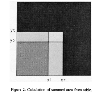
Assume the sum-table image is calculated. We need to know the sum of pixels of the original image that is defined by coordinates (xr, yt) and (xl,yb) on the illustration (brightest, smallest rectangle in the center). When we take the pixel value at the sum-table image at the location T(xr,yt) it would be the sum of all pixels in 4 bright rectangles. Then we subtract from it the sum of intensities of two rectangles (xr,yb) and (xl,yt) (just by reading the location from the sum-table image). Since they overlap, we subtracted the area in the rectangle (xk,yb) twice. So to get to the final result, we need to add the sum of (xk,yb) rectangle (again, by reading one value). The final formula from the cited paper is
T((xr, yt) / (xl,yb)) = T(xr, yt) – T(xr, yb) – T(xl,yt) + T(xl,yb).
So instead of iterating over all pixels of the rectangle, we got a sum in one go. To get the average value, dividing the sum by the area of the rectangle gives the average intensity over the rectangle.
For NCC, we want to calculate two integral sum-tables, one for the image itself and another one for the squared intensity values. Because in the denominator we need to calculate:
\(\sum_{x}[f(x)-\overline{f}_{x}]^2 = \sum_{x}[f(x)^2-2\overline{f}_{x} f(x)+\overline{f}_{x}^2] = -S\overline{f}_{x}^2 + \sum_{x}[f(x)^2]\)where S is the number of pixels in the overlapping region. So we take the average value from the first sum-table image and the sum of squared intensity values from the second.
The calculation of the sum-table image itself requires just \(O(N)\) complexity, so it is even faster than the numerator. We can perform pixel scanning and apply an inverse formula for obtaining sum values from above.
Having sum tables also speeds up the precise calculation of the numerator:
\(\displaystyle num(\Delta x) = \sum_{x}[f(x)-\overline{f}_{x}][g(x-\Delta x)-\overline{g}_{x}] =f(x)*g(x) – 2S\overline{f}_{x}\overline{g}_{x}+(\overline{f}_{x}\overline{g}_{x})^2\)
where the first term (convolution) is obtained using FFT.
This is a very efficient and widely used method. For example, that is how NCC is implemented in Matlab. In our lab, we used it as part of the Correlescence plugin for the analysis of spatiotemporal correlations of microscopy images.
At that point, it looked like the problem of slow NCC was solved.
But (as always) the devil is in the details. What is rarely mentioned is that this method is an approximation of the NCC. Meaning that it does not give exactly the same output as the direct method of computation. To add on top of that, specific implementations of this method are often pretty different since they depend on the application’s aim.
Let’s explore different NCC versions on one specific example image. The image is a kind of symmetric roof of a house. It is just 11×11 pixels (use this link to download the original), but I’ve scaled it up and color-coded using the viridis lookup table.

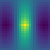
We are going to calculate auto-correlation, i.e., cross-correlation of the image with itself. I will disclose right away that this image was chosen specifically to highlight the limitations of the fast NCC calculation procedure. It was taken from masked NCC repo by Dirk Padfield (I am going to talk about it below). Here is the corresponding autocorrelation image, calculated using the direct NCC method.

As one can see, the NCC has a peak vertical line of value 1 at the center, since pixel intensities are constant along Y values. NCC is symmetric along the X shifts, with the correlation value decaying towards larger shifts.
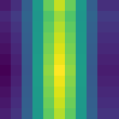
If we use Matlab’s normxcorr2 (from the image processing toolbox) function, the NCC looks completely different. The reason is that its implementation is simplified under the assumption that one image (the reference) is always much larger than the other (the template). It looks like this:
Not really what is expected. If I use my Correlescence plugin, the result is a bit better, but still not the same (and it returns only the central part of CC map by default):
In principle, this image can be used as a good test for any other correlation implementations. If you compare output CC maps using other, larger “regular” images, the difference is not so striking. Nevertheless, what is going on?
The answer lies in the Fourier transform, which these methods use. As mentioned above, the fast Fourier transform algorithm is used, and for the majority of its implementations (based on Cooley–Tukey method), it requires that the input image dimensions must be equal to a power of 2. And if the image has different dimensions, it is usually padded with zeros. This changes the original image (or function), especially since we need to subtract the average value at some point. Paddin introduces “tails” on the sides of images, and this leads to the artifacts in the final CC map, shown above. It is not a coincidence that the CC “breaking” image example above has dimensions of 11×11.
Generalized FFT form of NCC
At this point, it looked as if you want a precise NCC, the only way is to use the direct \(O(N^2)\) method. But things changed in 2011 (not so long ago), when Dirk Padfield published his paper “Masked Object Registration in the Fourier Domain” [matlab repo]. The details can be found there, but the main idea, as I understand it, is to use FFT not only on the padded numerator, but also to take “to Fourier space and back” the padded denominator. In this case, the output becomes indistinguishable to the direct NCC calculation method. From the calculation point of view, it is a bit heavier than fast NCC, since it requires six forward FFTs and six backwards FFTs (with some optimization). But it is still of \(O(N log N)\) order. The additional benefit of this is that the zero-padding can be used as a mask, telling NCC “to ignore” specific areas. Meaning that even if we have some images that are not rectangular (for example, from “triangular” ultrasound scans or square images that were polar transformed), we can mask-pad them with zeros and still register using this generalized NCC. I think this is pretty cool (and if Dirk is reading this post, kudos and hat off to you), and in principle, this implementation should be standard for NCC anywhere. It is part of scikit-image in Python, there is a C++ implementation, matlab code above. And of course, I’ve made a Fiji plugin out of it, AveragingND, where we use it to register arbitrary dimension/size images and it is part of iterative averaging.
That’s it! I hope you enjoyed the post!
0 Comments