//><=~!=//

It is not very clear, how biological systems (cells in particular) can bridge amazing ranges of scales in time and space.  To study these processes one would need a corresponding multi-scale measurement device (in theory). But microscope, for example, by default is one-scale instrument. Meaning that in 99% of movie acquisitions there is only one time scale. I mean frame rate, it is one of the major parameters (exposure in stream or the interval between frames in timelapse recording). So biological process that one can observe and record will highly depend on the chosen microscopy time-scale. If studied process happens on different time intervals, chances are one would miss it.

Now, the main question is how to pick the right timescale? So that you do not acquire too often on the one hand (and do not bleach your precious fluorophore) and not very rare so not to miss important changes. Can “best frame rate” be derived from operational principles of fluorescent microscope? Thinking about it I came up with this chart. It is mostly inspired by thinking about limits and picking up optimal conditions for single particle tracking.

 

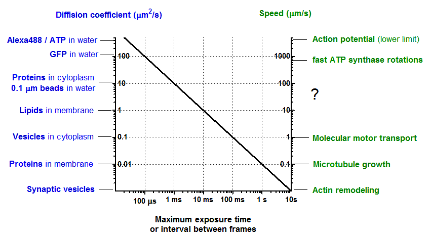
Here characteristics of “biological movement” are plotted on the y axis and the thick black curve projects them to the “optimal” framerate plotted at the x axis. On the left vertical axis I’ve plotted passive (diffusion) and active transport processes and estimated frame rate (exposure) needed to capture them before they would move for more then ~ 200 nm. Why this value? The majority of these processes are observed with fluorescent microscope and due to the diffraction limit particles will look like objects half of wavelength wide (and average of visible light is 500 nm). So if particle moves along distance longer than its own dimension during one frame acquisition , particle’s image is going to be smeared. It would not look like one bright spot, rather like a dim smear. And many moving particles will just create homogeneous bright background.

For 2D diffusion with coefficient this can be summarized by simple formula:

that is plotted above and looks like a straight line on log-log scale. Similar reasoning can be applied to processive motion with speed and in this case the formula is even more simple:

and kind of gives the same result.

Most of the time spent on this plot took a search for illustrative biological processes on both sides of the plot. First of all, I’m not absolutely sure that all estimations presented here are valid. It seems that in each case there are special cases and exceptions (well, as it is always in biology). The second interesting thing was that I don’t know any active subcellular biological process happening with speed in the range of 10-100 microns per second. Welcome to the low Reynolds number world? There are many on the level of organism, but subcellular? So this is why there is a question mark there.