//><=~!=//

In many areas of science (sociology, intracellular transport, stock exchange, climatology, etc) there is a need to decompose observed noisy time series into a set of piecewise linear trends. Let me show a typical example data that I’ve generated myself:

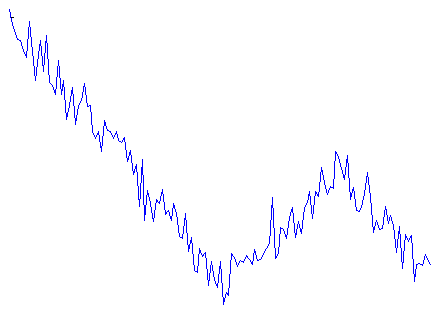
Time series of some signal representing miltiple linear trends with noise on top

Alternative to linear trends analysis method is Fourier transform (for example). But it assumes that the signal is periodic and the frequency spetrum is constant, so it usually works quite bad on the type of data shown above. For signals which change their scale/behaviour over time, most simple approximation is still piecewise linear approximation. Something like that (red dotted line is original signal before noise addition):

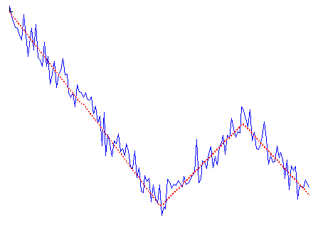
Combination of linear trends before (red dotted line) and after noise addition (blue solid line).

One of the best solutions for this task (in my opinion) is “Multiscale trend analysis” (MTA) approach developed in a series of papers from I. Zalyapin et al. [1], [2]. (actually it is much more than just finding linear approximations and I recommend to read papers to get it all)

It is very well described, but there is no available code, so I’ve wrote it in Matlab and decided to share. Here is example, how it works:

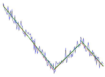
Combination of linear trends before (red dotted line) and after noise addition (blue solid line) and result of MTA algorithm (dark green solid line)

As can be seen, it does quite a good job. The crucial parameter is “when to stop fitting”, i.e. when the addition of new linear trends should stop. In the original paper the plot is built of rms difference between signal and different degrees approximations. The point where this curve changes it slope is considered optimal (in short). Since this approach seems to be a bit complicated to me, I’ve introduced another criteria: when the addition of new trend does not improve rms by more than X%, algorithm  stops. By default the value of the parameter is 5%, but one can change it to bigger/less value:

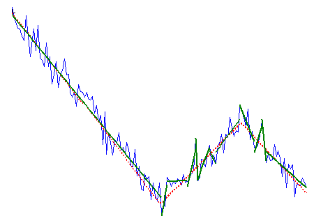
Overfitting

This is the case when the parameter value is 1% and so overfitting happens. The exact value for specific application can be quickly estimated by playing with data and it depends on the number of points per trend, noise level, etc.

I hope it will save some time for somebody and help with whatever research you are doing.